CS231n Assignments Note5: Convolutional Neural Network
Table of Contents:
- A Try to Interpret the Essence of A Convolutional Neural Network
- Layers Used to Build ConvNets
- Convolutional Layer
- Pooling Layer
- Layer Patterns
- Several Common Architecture
- Reference
A Try to Interpret the essence of A Convolutional Neural Network
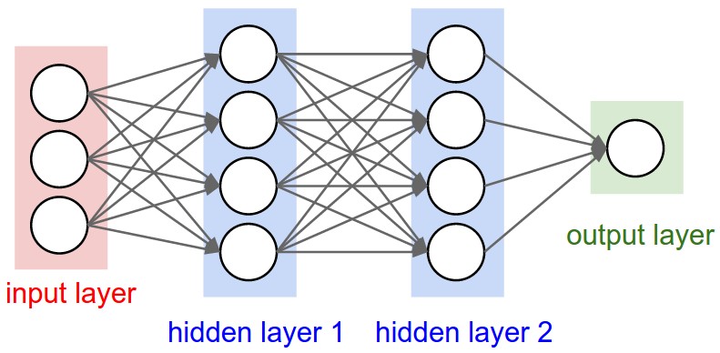
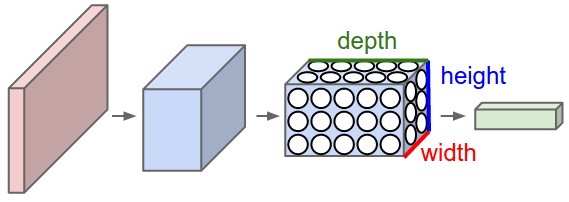
Left: A regular 3-layer Neural Network. Right: A ConvNet arranges its neurons in three dimensions (width, height, depth), as visualized in one of the layers. Every layer of a ConvNet transforms the 3D input volume to a 3D output volume of neuron activations. In this example, the red input layer holds the image, so its width and height would be the dimensions of the image, and the depth would be 3 (Red, Green, Blue channels).
ConvNet architectures make the explicit assumption that the inputs are images, which allows us to encode certain properties into the architecture. These then make the forward function more efficient to implement and vastly reduce the amount of parameters in the network.
The layers of a ConvNet have neurons arranged in 3 dimensions: width, height, depth. The neurons in a layer will only be connected to a small region of the layer before it, which finally make our model work much better.
A ConvNet is made up of Layers. Every Layer has a simple API: It transforms an input 3D volume to an output 3D volume with some differentiable function that may or may not have parameters.
Layers Used to Build ConvNets
We use three main types of layers to build ConvNet architectures: Convolutional Layer, Pooling Layer, and Fully-connected Layer. We stack these layers to form a full ConvNet architecture.
Example Architecture: [INPUT - CONV - RELU - POOL - FC]. In more detail:
- INPUT [32x32x3] will hold the raw pixel values of the image, in this case an image of width 32, height 32, and with three color channels R,G,B.
- CONV layer will compute the output of neurons that are connected to local regions in the input, each computing a dot product between their weights and a small region they are connected to in the input volume. This may result in volume such as [32x32x12] if we decided to use 12 filters.
- RELU layer will apply an elementwise activation function, such as the \(max(0,x)\) thresholding at zero. This leaves the size of the volume unchanged ([32x32x12]).
- POOL layer will perform a downsampling operation along the spatial dimensions (width, height), resulting in volume such as [16x16x12].
- FC (i.e. fully-connected) layer will compute the class scores, resulting in volume of size [1x1x10], where each of the 10 numbers correspond to a class score, such as among the 10 categories of CIFAR-10. As with ordinary Neural Networks and as the name implies, each neuron in this layer will be connected to all the numbers in the previous volume.
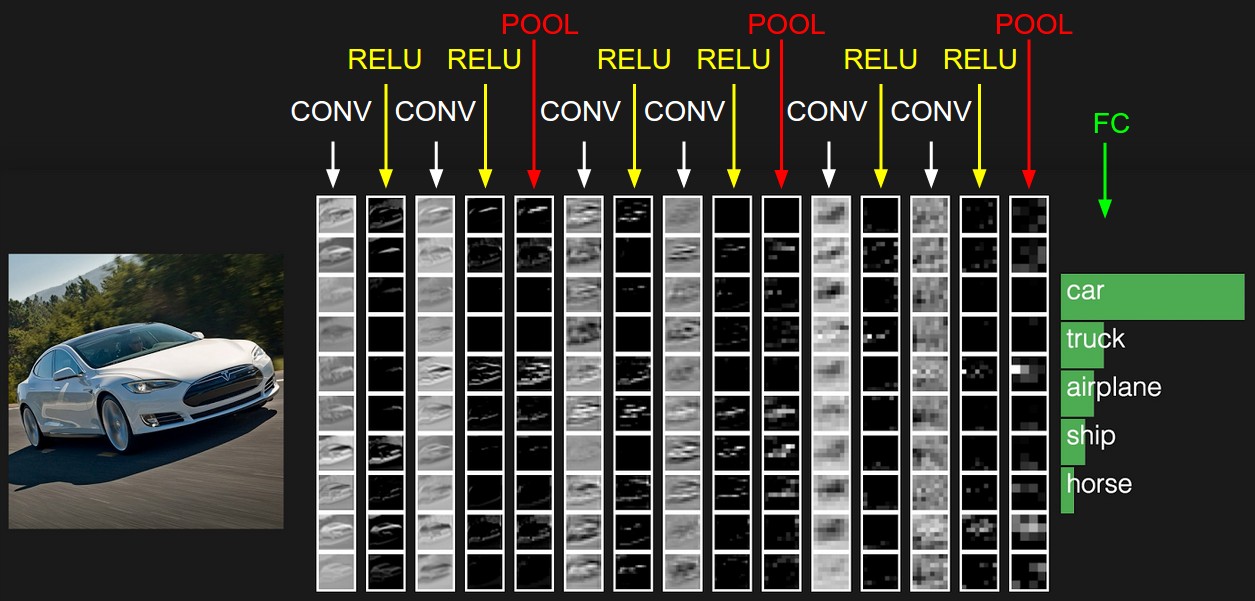
The activations of an example ConvNet architecture. The initial volume stores the raw image pixels (left) and the last volume stores the class scores (right). Each volume of activations along the processing path is shown as a column. Since it’s difficult to visualize 3D volumes, we lay out each volume’s slices in rows. The last layer volume holds the scores for each class, but here we only visualize the sorted top 5 scores, and print the labels of each one. The full web-based demo is shown in the header of our website. The architecture shown here is a tiny VGG Net, which we will discuss later.
Convolutional Layer
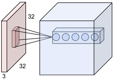
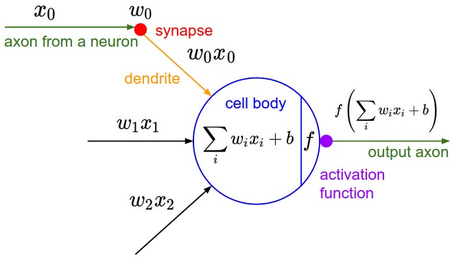
Left: An example input volume in red (e.g. a 32x32x3 CIFAR-10 image), and an example volume of neurons in the first Convolutional layer. Each neuron in the convolutional layer is connected only to a local region in the input volume spatially, but to the full depth (i.e. all color channels). Note, there are multiple neurons (5 in this example) along the depth, all looking at the same region in the input - see discussion of depth columns in text below. Right: The neurons from the Neural Network chapter remain unchanged: They still compute a dot product of their weights with the input followed by a non-linearity, but their connectivity is now restricted to be local spatially.
To make sense of the core block of ConvNet, convolutional layer, we must understand some important concept.
Filter(or Kernel). The CONV layer’s parameters consist of a set of learnable filters. Every filter is small spatially, but extends through the full depth of the input volume.
Receptive field. We connect each neuron to only a local region of the input volume. The spatial extent of this connectivity is a hyperparameter called the Receptive field.
Stride. We specify the stride to the number of pixels our filter slides. This is also a hyperparameter.
Zero-padding. It is a hyperparameter to pad the input volume with zeros around the border.
Make sure you understand this Convolution Demo. Below is a running demo of a CONV layer. Since 3D volumes are hard to visualize, all the volumes (the input volume (in blue), the weight volumes (in red), the output volume (in green)) are visualized with each depth slice stacked in rows. The input volume is of size \((W_1 = 5, H_1 = 5, D_1 = 3\)), and the CONV layer parameters are \((K = 2, F = 3, S = 2, P = 1\)). That is, we have two filters of size \((3 \times 3\)), and they are applied with a stride of 2. Therefore, the output volume size has spatial size (5 - 3 + 2)/2 + 1 = 3. Moreover, notice that a padding of \((P = 1\)) is applied to the input volume, making the outer border of the input volume zero. The visualization below iterates over the output activations (green), and shows that each element is computed by elementwise multiplying the highlighted input (blue) with the filter (red), summing it up, and then offsetting the result by the bias.
Pooling Layer
To progressively reduce the spatial size of the representation to reduce the amount of parameters and computation in the network, and hence to also control overfitting, it is common to periodically insert a pooling layre after CONV layers.
The most common form is a pooling layer with filters of size 2x2 applied with a stride of 2 downsamples every depth slice in the input by 2 along both width and height, discarding 75% of the activations. Every MAX operation would in this case be taking a max over 4 numbers (little 2x2 region in some depth slice). The depth dimension remains unchanged. More generally, the pooling layer:
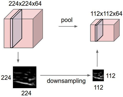
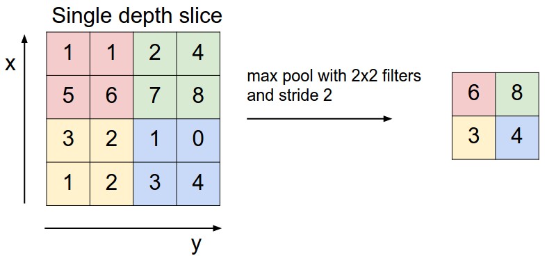
Pooling layer downsamples the volume spatially, independently in each depth slice of the input volume. Left: In this example, the input volume of size [224x224x64] is pooled with filter size 2, stride 2 into output volume of size [112x112x64]. Notice that the volume depth is preserved. Right: The most common downsampling operation is max, giving rise to max pooling, here shown with a stride of 2. That is, each max is taken over 4 numbers (little 2x2 square).
Note that many people dislike the pooling operation and think that we can get away without it.
Layer Patterns
The most common ConvNet architecture follows the pattern:
INPUT -> [[CONV -> RELU]*N -> POOL?]*M -> [FC -> RELU]*K - > FC
In practice: use whatever works best on ImageNet. If you’re feeling a bit of a fatigue in thinking about the architectural decisions, you’ll be pleased to know that in 90% or more of applications you should not have to worry about these. I like to summarize this point as “don’t be a hero”: Instead of rolling your own architecture for a problem, you should look at whatever architecture currently works best on ImageNet, download a pretrained model and finetune it on your data. You should rarely ever have to train a ConvNet from scratch or design one from scratch.
Several Common Architecture
There are several architectures in the field of Convolutional Networks that have a name. The most common are:
- LeNet. The first successful applications of Convolutional Networks were developed by Yann LeCun in 1990’s. Of these, the best known is the LeNet architecture that was used to read zip codes, digits, etc.
- AlexNet. The first work that popularized Convolutional Networks in Computer Vision was the AlexNet, developed by Alex Krizhevsky, Ilya Sutskever and Geoff Hinton. The AlexNet was submitted to the ImageNet ILSVRC challenge in 2012 and significantly outperformed the second runner-up (top 5 error of 16% compared to runner-up with 26% error). The Network had a very similar architecture to LeNet, but was deeper, bigger, and featured Convolutional Layers stacked on top of each other (previously it was common to only have a single CONV layer always immediately followed by a POOL layer).
- ZF Net. The ILSVRC 2013 winner was a Convolutional Network from Matthew Zeiler and Rob Fergus. It became known as the ZFNet (short for Zeiler & Fergus Net). It was an improvement on AlexNet by tweaking the architecture hyperparameters, in particular by expanding the size of the middle convolutional layers and making the stride and filter size on the first layer smaller.
- GoogLeNet. The ILSVRC 2014 winner was a Convolutional Network from Szegedy et al. from Google. Its main contribution was the development of an Inception Module that dramatically reduced the number of parameters in the network (4M, compared to AlexNet with 60M). Additionally, this paper uses Average Pooling instead of Fully Connected layers at the top of the ConvNet, eliminating a large amount of parameters that do not seem to matter much. There are also several followup versions to the GoogLeNet, most recently Inception-v4.
- VGGNet. The runner-up in ILSVRC 2014 was the network from Karen Simonyan and Andrew Zisserman that became known as the VGGNet. Its main contribution was in showing that the depth of the network is a critical component for good performance. Their final best network contains 16 CONV/FC layers and, appealingly, features an extremely homogeneous architecture that only performs 3x3 convolutions and 2x2 pooling from the beginning to the end. Their pretrained model is available for plug and play use in Caffe. A downside of the VGGNet is that it is more expensive to evaluate and uses a lot more memory and parameters (140M). Most of these parameters are in the first fully connected layer, and it was since found that these FC layers can be removed with no performance downgrade, significantly reducing the number of necessary parameters.
- ResNet. Residual Network developed by Kaiming He et al. was the winner of ILSVRC 2015. It features special skip connections and a heavy use of batch normalization. The architecture is also missing fully connected layers at the end of the network. The reader is also referred to Kaiming’s presentation (video, slides), and some recent experiments that reproduce these networks in Torch. ResNets are currently by far state of the art Convolutional Neural Network models and are the default choice for using ConvNets in practice (as of May 10, 2016). In particular, also see more recent developments that tweak the original architecture from Kaiming He et al. Identity Mappings in Deep Residual Networks (published March 2016).
Reference
Convolutional Neural Networks: Architectures, Convolution / Pooling Layers
Assignment #2: Fully-Connected Nets, Batch Normalization, Dropout, Convolutional Nets