CS231n Assignments Note2: Linear Classification of SVM and Softmax
Linear Classifier
Define a score function of linear classifier like this:
\[f(x_i, W, b) = W x_i + b\]Note that we can simplify the function:
\[f(x_i, W) = W x_i\]Take an image to interpret:
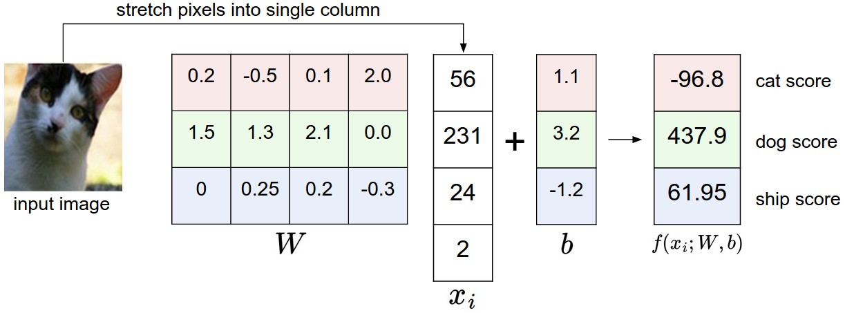
An example of mapping an image to class scores. For the sake of visualization, we assume the image only has 4 pixels (4 monochrome pixels, we are not considering color channels in this example for brevity), and that we have 3 classes (red (cat), green (dog), blue (ship) class). (Clarification: in particular, the colors here simply indicate 3 classes and are not related to the RGB channels.) We stretch the image pixels into a column and perform matrix multiplication to get the scores for each class. Note that this particular set of weights W is not good at all: the weights assign our cat image a very low cat score. In particular, this set of weights seems convinced that it’s looking at a dog.
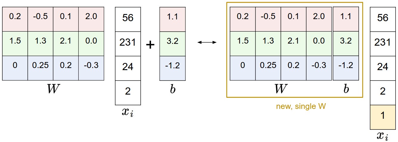
Illustration of the bias trick. Doing a matrix multiplication and then adding a bias vector (left) is equivalent to adding a bias dimension with a constant of 1 to all input vectors and extending the weight matrix by 1 column - a bias column (right). Thus, if we preprocess our data by appending ones to all vectors we only have to learn a single matrix of weights instead of two matrices that hold the weights and the biases.
Analogy of images as high-dimensional points. As the following picture shows, every row of parameter $ W $ is a classifier for one of the classes.
![]()
Cartoon representation of the image space, where each image is a single point, and three classifiers are visualized. Using the example of the car classifier (in red), the red line shows all points in the space that get a score of zero for the car class. The red arrow shows the direction of increase, so all points to the right of the red line have positive (and linearly increasing) scores, and all points to the left have a negative (and linearly decreasing) scores.
Linear classifier as template matching. We can also interpret each row of $ W $ as template for one of the classes as the picture shows below:
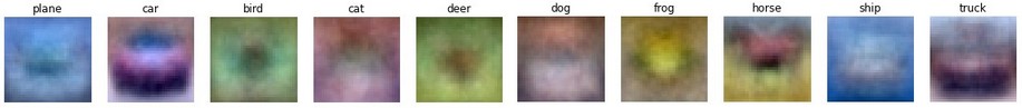
Skipping ahead a bit: Example learned weights at the end of learning for CIFAR-10. Note that, for example, the ship template contains a lot of blue pixels as expected. This template will therefore give a high score once it is matched against images of ships on the ocean with an inner product.
Support Vector Machine(SVM)
Multiclass Support Machine loss function is formalized as follows:
\[L_i = \sum_{j\neq y_i} \max(0, s_j - s_{y_i} + \Delta)\]where $ s = f(x_i, W) $. The loss function wants the scores of the correct class $ y_i $ to be larger than incorrect class scores by at least $ \Delta $.
For a more explicit way to write this function:
\[L_i = \sum_{j\neq y_i} \max(0, w_j^T x_i - w_{y_i}^T x_i + \Delta)\]where we call $ max(0,-) $ as hinge loss, $ max(0,-)^2 $ as squared hinge loss(or L2-SVM).
Here are two ways of implements:
def svm_loss_naive(W, X, y, reg):
    """
    Structured SVM loss function, naive implementation (with loops).

    Inputs have dimension D, there are C classes, and we operate on minibatches
    of N examples.

    Inputs:
    - W: A numpy array of shape (D, C) containing weights.
    - X: A numpy array of shape (N, D) containing a minibatch of data.
    - y: A numpy array of shape (N,) containing training labels; y[i] = c means
      that X[i] has label c, where 0 <= c < C.
    - reg: (float) regularization strength

    Returns a tuple of:
    - loss as single float
    - gradient with respect to weights W; an array of same shape as W
    """
    dW = np.zeros(W.shape) # initialize the gradient as zero

        #############################################################################
    # TODO:                                                                     #
    # Compute the gradient of the loss function and store it dW.                #
    # Rather that first computing the loss and then computing the derivative,   #
    # it may be simpler to compute the derivative at the same time that the     #
    # loss is being computed. As a result you may need to modify some of the    #
    # code above to compute the gradient.                                       #
    #############################################################################
    # *****START OF YOUR CODE (DO NOT DELETE/MODIFY THIS LINE)*****

    #for i in range(num_train):
    #    scores = X[i].dot(W)
    #    correct_class_score = scores[y[i]]
    #    for j in range(num_classes):
    #        if j == y[i]:
    #            continue
    #        margin = scores[j] - correct_class_score + 1 # note delta = 1
    #        if margin > 0:

    # compute the loss and the gradient
    num_classes = W.shape[1]
    num_train = X.shape[0]
    loss = 0.0
    for i in range(num_train):
        scores = X[i].dot(W)
        correct_class_score = scores[y[i]]
        for j in range(num_classes):
            if j == y[i]:
                continue
            margin = scores[j] - correct_class_score + 1 # note delta = 1
            if margin > 0:
                loss += margin
                dW[:,y[i]] -= X[i,:].T
                dW[:,j] += X[i,:].T

    # Right now the loss is a sum over all training examples, but we want it
    # to be an average instead so we divide by num_train.
    loss /= num_train
    dW /= num_train

    # Add regularization to the loss.
    loss += reg * np.sum(W * W)
    dW += 2 * reg * W


    # *****END OF YOUR CODE (DO NOT DELETE/MODIFY THIS LINE)*****

    return loss, dW


def svm_loss_vectorized(W, X, y, reg):
    """
    Structured SVM loss function, vectorized implementation.

    Inputs and outputs are the same as svm_loss_naive.
    """
    num_classes = W.shape[1]
    num_train = X.shape[0]

    loss = 0.0
    dW = np.zeros(W.shape) # initialize the gradient as zero

    #############################################################################
    # TODO:                                                                     #
    # Implement a vectorized version of the structured SVM loss, storing the    #
    # result in loss.                                                           #
    #############################################################################
    # *****START OF YOUR CODE (DO NOT DELETE/MODIFY THIS LINE)*****

    delta = 1.0
    scores = X.dot(W)
    scores_corr = scores[np.arange(num_train), y].reshape((num_train, -1))
    margins = np.maximum(0, scores - scores_corr + delta)
    margins[np.arange(num_train), y] = 0
    loss = np.sum(margins) / num_train
    loss += reg * np.sum(W * W)

    # *****END OF YOUR CODE (DO NOT DELETE/MODIFY THIS LINE)*****

    #############################################################################
    # TODO:                                                                     #
    # Implement a vectorized version of the gradient for the structured SVM     #
    # loss, storing the result in dW.                                           #
    #                                                                           #
    # Hint: Instead of computing the gradient from scratch, it may be easier    #
    # to reuse some of the intermediate values that you used to compute the     #
    # loss.                                                                     #
    #############################################################################
    # *****START OF YOUR CODE (DO NOT DELETE/MODIFY THIS LINE)*****

    # Shape of margin: N X C
    #for i in range(num_train):
    #    for j in range(num_classes):
    #        if margins[i][j] > 0:
    #            dW[:,y[i]] -= X[i,:]
    #            dW[:,j] += X[i,:]
    # dW /= num_train
    # dW += 2 * reg * W
    margins[margins>0]=1.0
    row_sum = np.sum(margins,axis=1)
    # for i in range(margins.shape[1]):
    #     margins[:, i] *= row_sum
    margins[np.arange(num_train),y] = -row_sum
    dW = np.dot(X.T,margins) / num_train + 2 * reg*W;

    # *****END OF YOUR CODE (DO NOT DELETE/MODIFY THIS LINE)*****

    return loss, dW
-
Especially note that the code of the vectorized version, it is simple but kind of confused to make sense.
-
Note that it is different between
margins[y]andmargins[np.arange(num_train), y].
Softmax
Define cross-entropy loss having the form:
\[L_i = -\log\left(\frac{e^{f_{y_i}}}{ \sum_j e^{f_j} }\right) \hspace{0.5in} \text{or equivalently} \hspace{0.5in} L_i = -f_{y_i} + \log\sum_j e^{f_j}\]where the function The function \(f_j(z) = \frac{e^{z_j}}{\sum_k e^{z_k}} \) is called the softmax function
Look at the expression:
\[P(y_i \mid x_i; W) = \frac{e^{f_{y_i}}}{\sum_j e^{f_j} }\]a probabilistic interpretion says that the probability is assigned to the correct label $ y_i $ given the image $ x_i $ and parameterized by $ W $.
Two ways of implements using python:
def softmax_loss_naive(W, X, y, reg):
    """
    Softmax loss function, naive implementation (with loops)

    Inputs have dimension D, there are C classes, and we operate on minibatches
    of N examples.

    Inputs:
    - W: A numpy array of shape (D, C) containing weights.
    - X: A numpy array of shape (N, D) containing a minibatch of data.
    - y: A numpy array of shape (N,) containing training labels; y[i] = c means
      that X[i] has label c, where 0 <= c < C.
    - reg: (float) regularization strength

    Returns a tuple of:
    - loss as single float
    - gradient with respect to weights W; an array of same shape as W
    """
    # Initialize the loss and gradient to zero.
    loss = 0.0
    dW = np.zeros_like(W)

    #############################################################################
    # TODO: Compute the softmax loss and its gradient using explicit loops.     #
    # Store the loss in loss and the gradient in dW. If you are not careful     #
    # here, it is easy to run into numeric instability. Don't forget the        #
    # regularization!                                                           #
    #############################################################################
    # *****START OF YOUR CODE (DO NOT DELETE/MODIFY THIS LINE)*****

    for i in range(X.shape[0]):
        score = X[i].dot(W)
        score -= np.max(score)
        log_term = np.sum(np.exp(score))
        loss += - score[y[i]] + np.log(log_term)
        for j in range(W.shape[1]):
            ds = np.exp(score[j]) / log_term
            if j == y[i]:
                dW[:,j] += (ds - 1) * X[i,:].T
            else:
                dW[:,j] += ds * X[i,:].T

    loss /= X.shape[0]
    loss += reg * np.sum(W * W)
    dW /= X.shape[0]
    dW += 2 * reg * W


        # *****END OF YOUR CODE (DO NOT DELETE/MODIFY THIS LINE)*****

    return loss, dW


def softmax_loss_vectorized(W, X, y, reg):
    """
    Softmax loss function, vectorized version.

    Inputs and outputs are the same as softmax_loss_naive.
    """
    # Initialize the loss and gradient to zero.
    loss = 0.0
    dW = np.zeros_like(W)

    #############################################################################
    # TODO: Compute the softmax loss and its gradient using no explicit loops.  #
    # Store the loss in loss and the gradient in dW. If you are not careful     #
    # here, it is easy to run into numeric instability. Don't forget the        #
    # regularization!                                                           #
    #############################################################################
    # *****START OF YOUR CODE (DO NOT DELETE/MODIFY THIS LINE)*****

    score = X.dot(W)
    score -= np.max(score)
    log_term = np.sum(np.exp(score), axis=1)
    loss = np.sum(- score[np.arange(X.shape[0]), y] +
            np.log(log_term))
    index = np.zeros_like(score)
    index[np.arange(X.shape[0]), y] = 1
    ds = np.exp(score) / log_term.reshape(X.shape[0], 1)
    dW = X.T.dot(ds - index)
    #dW[np.arange(W.shape[0]), y] = X.T.dot(ds - 1)

    loss /= X.shape[0]
    loss += reg * np.sum(W * W)
    dW /= X.shape[0]
    dW += 2 * reg * W


    # *****END OF YOUR CODE (DO NOT DELETE/MODIFY THIS LINE)*****

    return loss, dW
- Similarly note how the vectorized version is implemented.
- This blog is helpful for understanding calculation of the gradient.
A Detail
A interesting detail I want to note is that I mix the following codes when writing codes to fetch batch of training sets fot doing SGD:
X_batch = X[np.random.choice(np.arange(num_train), batch_size, replace=True)]
y_batch = y[np.random.choice(np.arange(num_train), batch_size, replace=True)]
This is wrong because X_batch does not match y_batch to form training sets. The right version should like this:
mask = np.random.choice(np.arange(num_train), batch_size, replace=True)
X_batch = X[mask]
y_batch = y[mask]
Reference
Linear classification: Support Vector Machine, Softmax
Optimization: Stochastic Gradient Descent
Assignment #1: Image Classification, kNN, SVM, Softmax, Neural Network