Bayesian Optimization
Table of contens:
Solving problem $\max _{x \in A} f(x)$, Bayesian Optimization(BO) is a good choice if:
-
The input $x$ is in low dimension, typically $d \leq 20$;
-
$f$ is “expensive” to evaluate/query;
-
$f$ is black-box
Bayesian Optimization consists of two main components:
- Bayesian statistical model
- Aquisition function
Bayesian statistical model(Surrogate model)
Statistical model is used for approximating the objective function: it provides a Bayesian posterior probability distribution that describes potential values for the objective function at any candidate point. This posterior distribution is updated each time we query the objective function at a new point. Generally we use Gaussian Process(GP) as statistical model. Model the objective function $h$:
\[h \sim \mathcal{N}\left(\mu_{0}, \Sigma_{0}\right)\]where $\mu_{0}$ is typically constant mean function: $ \mu_{0} = \mu $, covariance function $\Sigma_{0}$ is typically defined as:
\[\Sigma_{0}\left(\mathbf{x}, \mathbf{x}^{\prime}\right)=\theta_{0}^{2} \exp (-\sqrt{5} r)\left(1+\sqrt{5} r+\frac{5}{3} r^{2}\right), \quad r^{2}=\sum_{i=1}^{d^{\prime}} \frac{\left(x_{i}-x_{i}^{\prime}\right)^{2}}{\theta_{i}^{2}}\]Acquisition Function
We use acquisition function $\mathcal{A}$ to get a new point based on statistical model that has taken some points to update:
\[x_{new}=\arg \max _{x} \mathcal{A}(\mu,\sigma^{2},x)\]One of mostly chosen acquisition function is Expected Improvement(EI):
\[E I(x)=\left\{\begin{array}{ll}\left(\mu(x)-f\left(x^{+}\right)\right) \Phi(z)+\sigma(x) \Phi(z) & \sigma>0 \\ 0 & \sigma=0\end{array}\right.\] \[z=\frac{\mu(x)-f\left(x^{+}\right)}{\sigma}\]General Algorithm
workflow
Complete algorithm can be described like this:
-
初始化计算$k$个点:$\mathcal{D} = {(x_{1}, f\left(x_{1}\right)), \ldots, (x_{k}, f\left(x_{k}\right))}$, 其中$x_{1}, \ldots, x_{k} \in \mathbb{R}^{d}$
-
用一个统计模型GP模拟(modeling)目标函数,先验分布:\(f\left(x_{1: k}\right) \sim \operatorname{Normal}\left(\mu_{0}\left(x_{1: k}\right), \Sigma_{0}\left(x_{1: k}, x_{1: k}\right)\right)\)
-
根据GP的均值$\mu$和方差$\sigma^{2}$,求得此时的提取函数(EI)进而得到EI最大值对应的点:\(x_{new}=\arg \max _{x} \mathrm{EI}(\mu,\sigma^{2},x)\)
-
观察点$(x_{new}, f\left(x_{new}\right))$;
-
如果满足要求(查询次数或最优点),返回;否则,$\mathcal{D} \leftarrow \mathcal{D} \cup(x_{new}, f\left(x_{new}\right))$,更新GP,回到第3步.
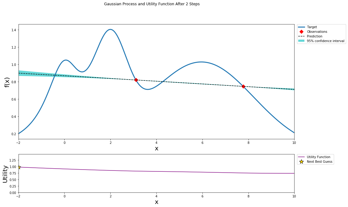
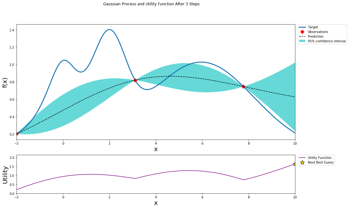
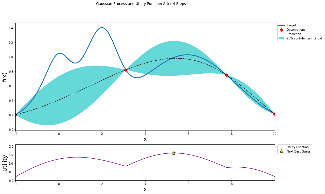
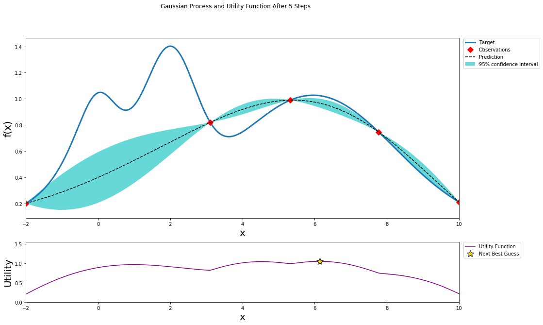
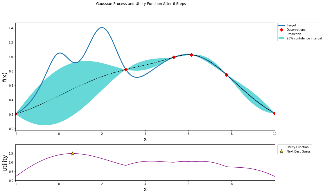
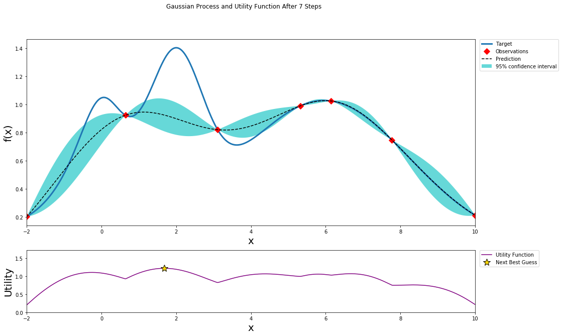
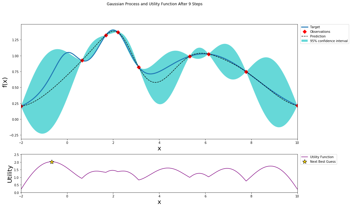
better understanding
This github repo and blog give a clear visual process of how Bayesian Optimization works: